26. Libraries and Modules

A library is a collection of code for functions and classes. Often, these libraries are written by someone else and brought into the project so that the programmer does not have to “reinvent the wheel.” In Python the term used to describe a library of code is module.
By using import arcade and import random, the programs created so far have
already used modules. A library can be made up of multiple modules that can be
imported. Often a library only has one module, so these words can sometimes be
used interchangeably.
Modules are often organized into groups of similar functionality. In this class
programs have already used functions from the math module, the random module,
and the arcade library. Modules can be organized so that individual modules
contain other modules. For example, the arcade module contains submodules for
arcade.key, and arcade.color.
Modules are not loaded unless the program asks them to. This saves time and computer memory. This chapter shows how to create a module, and how to import and use that module.
26.1. Why Create a Library?
There are three major reasons for a programmer to create his or her own libraries:
It breaks the code into smaller, easier to use parts.
It allows multiple people to work on a program at the same time.
The code written can be easily shared with other programmers.
Some of the programs already created in this book have started to get rather long. By separating a large program into several smaller programs, it is easier to manage the code. For example, in the prior chapter’s sprite example, a programmer could move the sprite class into a separate file. In a complex program, each sprite might be contained in its own file.
If multiple programmers work on the same project, it is nearly impossible to do so if all the code is in one file. However, by breaking the program into multiple pieces, it becomes easier. One programmer could work on developing an “Orc” sprite class. Another programmer could work on the “Goblin” sprite class. Since the sprites are in separate files, the programmers do not run into conflict.
Modern programmers rarely build programs from scratch. Often programs are built from parts of other programs that share the same functionality. If one programmer creates code that can handle a mortgage application form, that code will ideally go into a library. Then any other program that needs to manage a mortgage application form at that bank can call on that library.
26.2. Creating Your Own Module/Library File
Video: Libraries
In this example we will break apart a short program into multiple files. Here
we have a function in a file named test.py, and a call to that function:
1 2 3 4 5 6 7 8 9 | # Foo function
def foo():
print("foo!")
def main():
# Foo call
foo()
main()
|
Yes, this program is not too long to be in one file. But if both the function and the main program code were long, it would be different. If we had several functions, each 100 lines long, it would be time consuming to manage that large of a file. But for this example we will keep the code short for clarity.
We can move the foo function out of this file. Then this file would be left
with only the main program code. (In this example there is no reason to
separate them, aside from learning how to do so.)
To do this, create a new file and copy the foo function into it. Save the
new file with the name my_functions.py. The file must be saved to the same
directory as test.py.
1 2 3 | # Foo function
def foo():
print("foo!")
|
1 2 3 4 5 | def main():
# Foo call that doesn't work
foo()
main()
|
Unfortunately it isn’t as simple as this. The file test.py does not know to
go and look at the my_functions.py file and import it. We have to add the
command to import it:
1 2 3 4 5 6 7 8 | # Import the my_functions.py file
import my_functions
def main():
# Foo call that still doesn't work
foo()
main()
|
That still doesn’t work. What are we missing? Just like when we import arcade, we have to put the package name in front of the function. Like this:
1 2 3 4 5 6 7 8 | # Import the my_functions.py file
import my_functions
def main():
# Foo call that does work
my_functions.foo()
main()
|
This works because my_functions. is prepended to the function call.
26.3. Namespace
Video: Namespace
A program might have two library files that need to be used. What if the libraries had functions that were named the same? What if there were two functions named print_report, one that printed grades, and one that printed an account statement? For instance:
1 2 | def print_report():
print("Student Grade Report:" )
|
1 2 | def print_report():
print("Financial Report:" )
|
How do you get a program to specify which function to call? Well, that is pretty easy. You specify the namespace. The namespace is the work that appears before the function name in the code below:
1 2 3 4 5 6 7 8 | import student_functions
import financial_functions
def main():
student_functions.print_report()
financial_functions.print_report()
main()
|
So now we can see why this might be needed. But what if you don’t have name
collisions? Typing in a namespace each and every time can be tiresome. You
can get around this by importing the library into the local namespace. The
local namespace is a list of functions, variables, and classes that you
don’t have to prepend with a namespace. Going back to the foo example,
let’s remove the original import and replace it with a new type of import:
1 2 3 4 5 6 7 | # import foo
from my_functions import *
def main():
foo()
main()
|
This works even without my_functions. prepended to the function call. The
asterisk is a wildcard that will import all functions from my_functions.
A programmer could import individual ones if desired by specifying the
function name.
26.4. Third Party Libraries
When working with Python, it is possible to use many libraries that are built into Python. Take a look at all the libraries that are available here:
http://docs.python.org/3/py-modindex.html
It is possible to download and install other libraries. There are libraries that work with the web, complex numbers, databases, and more.
Arcade: The library that this book uses to create games. http://arcade.academy
Pygame: Another library used to create games, and the inspiration behind the creation of the Arcade library. http://www.pygame.org/docs/
Pymunk: A great library for running 2D physics. Also works with Arcade, see these examples http://www.pymunk.org/
wxPython: Create GUI programs, with windows, menus, and more. http://www.wxpython.org/
pydot: Generate complex directed and non-directed graphs http://code.google.com/p/pydot/
NumPy: Sophisticated library for working with matrices. http://numpy.org/
Pandas: A library for data analysis. https://pandas.pydata.org/
Pillow: Work with images. https://pillow.readthedocs.io/en/latest/
Pyglet: Another graphics library. Arcade uses this library. http://pyglet.org/
You can do analysis and create your own interactive notebook using Jupyter:
Jupyter: http://jupyter.org/
Some libraries we give examples of in this chapter:
OpenPyXL: A library for reading and writing Excel files. https://openpyxl.readthedocs.io/en/stable/
Beautiful Soup: Grab data off websites, and create your own web bots. https://www.crummy.com/software/BeautifulSoup/
MatPlotLib: Plot data automatically: https://matplotlib.org/
A wonderful list of Python libraries and links to installers for them is available here:
You can search up some top packages/libraries and stand alone projects to get an idea of what you can do. There are many articles like Top 15 Python Libraries for Data Science in 2017.
26.4.1. Examples: OpenPyXL Library
This example uses a library called OpenPyXL to write an Excel file. It is also
easy to read from an Excel file.
You can install OpenPyXL from the Windows command prompt by typing
pip install openpyxl.
If you are on the Mac or a Linux machine, you can type sudo pip3 install openpyxl.
Note
When starting the command prompt, you might need to right-click on it and select “Run as administrator” if you get permission errors when installing. And if you are working on a lab computer, you might not have permission to install libraries.
1 2 3 4 5 6 7 8 9 10 11 12 13 14 15 16 17 18 19 20 21 22 | """
Example using OpenPyXL to create an Excel worksheet
"""
from openpyxl import Workbook
import random
# Create an Excel workbook
work_book = Workbook()
# Grab the active worksheet
work_sheet = work_book.active
# Data can be assigned directly to cells
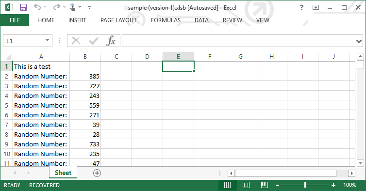
work_sheet['A1'] = "This is a test"
# Rows can also be appended
for i in range(200):
work_sheet.append(["Random Number:", random.randrange(1000)])
# Save the file
work_book.save("sample.xlsx")
|
The output of this program is an Excel file:
26.4.2. Examples: Beautiful Soup Library
This example grabs information off a web page.
You can install Beautiful Soup from the Windows command prompt by typing
pip install bs4. If you are on the Mac or a Linux machine, you can type
sudo pip3 install bs4.
1 2 3 4 5 6 7 8 9 10 11 12 13 14 15 16 17 18 19 20 | """
Example showing how to read in from a web page
"""
from bs4 import BeautifulSoup
import urllib.request
# Read in the web page
url_address = "http://simpson.edu"
page = urllib.request.urlopen(url_address)
# Parse the web page
soup = BeautifulSoup(page.read(), "html.parser")
# Get a list of level 1 headings in the page
headings = soup.findAll("h1")
# Loop through each row
for heading in headings:
print(heading.text)
|
26.4.3. Examples: Matplotlib Library
Here is an example of what you can do with the third party library “Matplotlib.”
You can install Matplotlib from the Windows command prompt by typing
pip install matplotlib. If you are on the Mac or a Linux machine, you can
type pip3 install matplotlib.
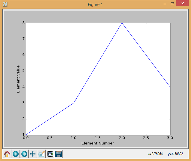
26.4.3.1. Example 1: Simple Plot
To start with, here is the code to create a simple line chart with four values:
Simple Line Graph
1 2 3 4 5 6 7 8 9 10 11 12 13 | """
Line chart with four values.
The x-axis defaults to start at zero.
"""
import matplotlib.pyplot as plt
y = [1, 3, 8, 4]
plt.plot(y)
plt.ylabel('Element Value')
plt.xlabel('Element Number')
plt.show()
|
Note that you can zoom in, pan, and save the graph. You can even save the graph in vector formats like ps and svg that import into documents without loss of quality like raster graphics would have.
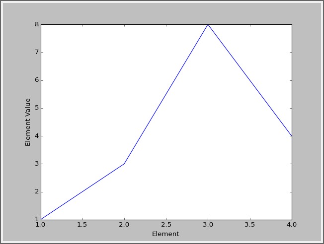
26.4.3.2. Example 2: Specify x Values
The x value for Example 1, defaults to start at zero. You can change this default and specify your own x values to go with the y values. See Example 2 below.
Specifying the x values
1 2 3 4 5 6 7 8 9 10 11 12 13 14 15 | """
Line chart with four values.
The x-axis values are specified as well.
"""
import matplotlib.pyplot as plt
x = [1, 2, 3, 4]
y = [1, 3, 8, 4]
plt.plot(x, y)
plt.ylabel('Element Value')
plt.xlabel('Element')
plt.show()
|
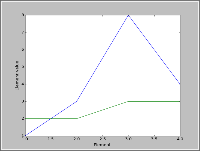
26.4.3.3. Example 3: Add A Second Data Series
It is trivial to add another data series to the graph.
Graphing two data series
1 2 3 4 5 6 7 8 9 10 11 12 13 14 15 16 17 18 | """
This example shows graphing two different series
on the same graph.
"""
import matplotlib.pyplot as plt
x = [1, 2, 3, 4]
y1 = [1, 3, 8, 4]
y2 = [2, 2, 3, 3]
plt.plot(x, y1)
plt.plot(x, y2)
plt.ylabel('Element Value')
plt.xlabel('Element')
plt.show()
|
26.4.3.4. Example 4: Add A Legend
You can add a legend to the graph:
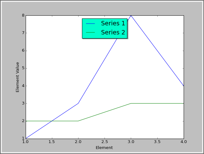
Adding a legend
1 2 3 4 5 6 7 8 9 10 11 12 13 14 15 16 17 |
import matplotlib.pyplot as plt

x =  [1, 2, 3, 4]
y1 = [1, 3, 8, 4]
y2 = [2, 2, 3, 3]

plt.plot(x, y1, label = "Series 1")
plt.plot(x, y2, label = "Series 2")

legend = plt.legend(loc='upper center', shadow=True, fontsize='x-large')
legend.get_frame().set_facecolor('#00FFCC')

plt.ylabel('Element Value')
plt.xlabel('Element')

plt.show()
|
26.4.3.5. Example 5: Add Annotations
You can add annotations to a graph:
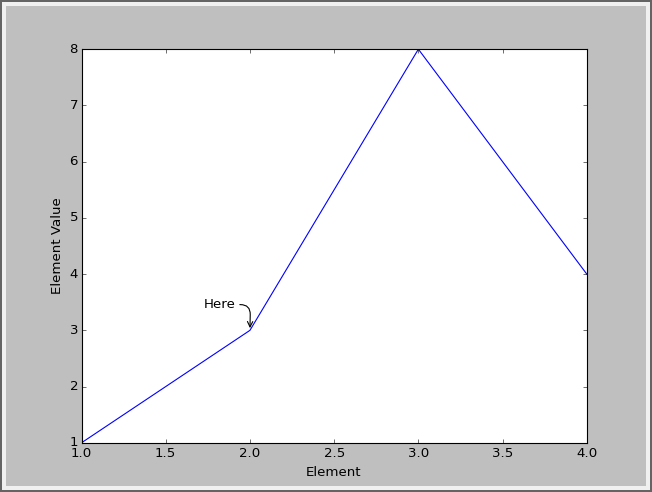
Adding annotations
1 2 3 4 5 6 7 8 9 10 11 12 13 14 15 16 17 18 19 20 21 22 23 | """
Annotating a graph
"""
import matplotlib.pyplot as plt
x = [1, 2, 3, 4]
y = [1, 3, 8, 4]
plt.annotate('Here',
xy = (2, 3),
xycoords = 'data',
xytext = (-40, 20),
textcoords = 'offset points',
arrowprops = dict(arrowstyle="->",
connectionstyle="arc,angleA=0,armA=30,rad=10"),
)
plt.plot(x, y)
plt.ylabel('Element Value')
plt.xlabel('Element')
plt.show()
|
26.4.3.6. Example 6: Change Line Styles
Don’t like the default lines styles for the graph? That can be changed by adding a third parameter to the plot command.
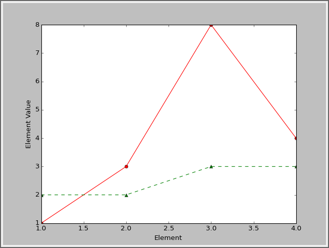
Specifying the line style
1 2 3 4 5 6 7 8 9 10 11 12 13 14 15 16 17 18 19 20 21 22 23 24 25 | """
This shows how to set line style and markers.
"""
import matplotlib.pyplot as plt
x = [1, 2, 3, 4]
y1 = [1, 3, 8, 4]
y2 = [2, 2, 3, 3]
# First character: Line style
# One of '-', '--', '-.', ':', 'None', ' ', "
# Second character: color
# http://matplotlib.org/1.4.2/api/colors_api.html
# Third character: marker shape
# http://matplotlib.org/1.4.2/api/markers_api.html
plt.plot(x, y1, '-ro')
plt.plot(x, y2, '--g^')
plt.ylabel('Element Value')
plt.xlabel('Element')
plt.show()
|
26.4.3.7. Example 7: Bar Chart
A bar chart is as easy as changing plot to bar.
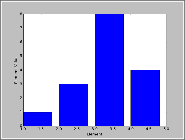
Bar chart
1 2 3 4 5 6 7 8 9 10 11 12 13 14 | """
How to do a bar chart.
"""
import matplotlib.pyplot as plt
x = [1, 2, 3, 4]
y = [1, 3, 8, 4]
plt.bar(x, y)
plt.ylabel('Element Value')
plt.xlabel('Element')
plt.show()
|
26.4.3.8. Example 8: Axis Labels
You can add labels to axis values.
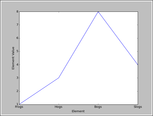
X-axis labels
1 2 3 4 5 6 7 8 9 10 11 12 13 14 15 16 17 | """
How to add x axis value labels.
"""
import matplotlib.pyplot as plt
x = [1, 2, 3, 4]
y = [1, 3, 8, 4]
plt.plot(x, y)
labels = ['Frogs', 'Hogs', 'Bogs', 'Slogs']
plt.xticks(x, labels)
plt.ylabel('Element Value')
plt.xlabel('Element')
plt.show()
|
26.4.3.9. Example 9: Graph Functions
You can graph functions as well. This uses a different package called numpy to graph a sine function.
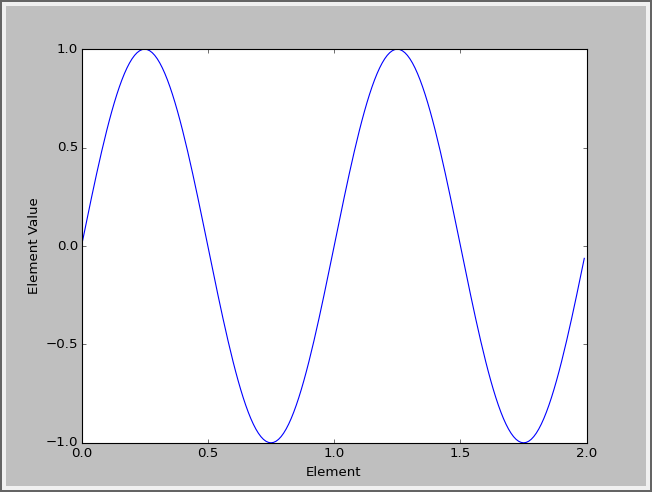
Graphing a sine function
1 2 3 4 5 6 7 8 9 10 11 12 13 14 15 16 | """
Using the numpy package to graph a function over
a range of values.
"""
import numpy
import matplotlib.pyplot as plt
x = numpy.arange(0.0, 2.0, 0.001)
y = numpy.sin(2 * numpy.pi * x)
plt.plot(x, y)
plt.ylabel('Element Value')
plt.xlabel('Element')
plt.show()
|
26.4.3.10. Example 10: Graph Functions With Fill
You can fill in a graph if you like.
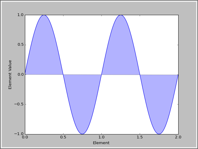
Filling in a graph
1 2 3 4 5 6 7 8 9 10 11 12 13 14 15 16 17 18 | """
Using 'fill' to fill in a graph
"""
import numpy
import matplotlib.pyplot as plt
x = numpy.arange(0.0, 2.0, 0.001)
y = numpy.sin(2 * numpy.pi * x)
plt.plot(x, y)
# 'b' means blue. 'alpha' is the transparency.
plt.fill(x, y, 'b', alpha=0.3)
plt.ylabel('Element Value')
plt.xlabel('Element')
plt.show()
|
26.4.3.11. Example 11: Pie Chart
Create a pie chart.
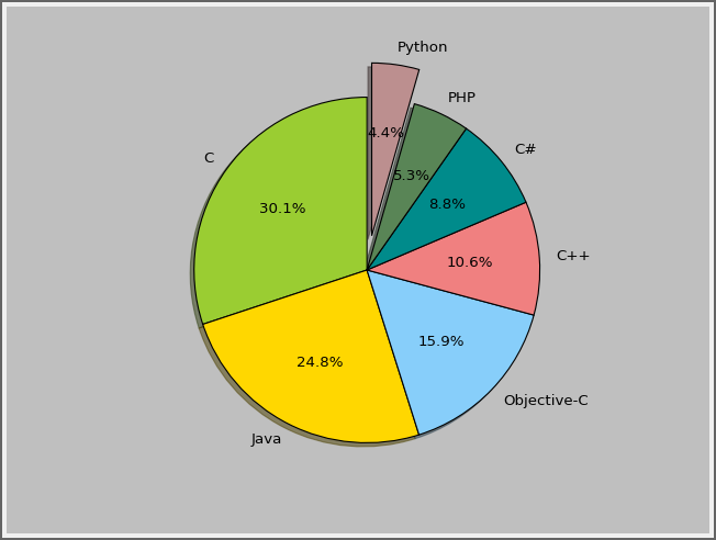
Pie chart
1 2 3 4 5 6 7 8 9 10 11 12 13 14 15 16 17 18 19 20 21 22 23 24 25 26 | """
Create a pie chart
"""
import matplotlib.pyplot as plt
# Labels for the pie chart
labels = ['C', 'Java', 'Objective-C', 'C++', 'C#', 'PHP', 'Python']
# Sizes for each label. We use this to make a percent
sizes = [17, 14, 9, 6, 5, 3, 2.5]
# For list of colors, see:
# https://matplotlib.org/examples/color/named_colors.html
colors = ['yellowgreen', 'gold', 'lightskyblue', 'lightcoral', 'darkcyan', 'aquamarine', 'rosybrown']
# How far out to pull a slice. Normally zero.
explode = (0, 0.0, 0, 0, 0, 0, 0.2)
# Set aspect ratio to be equal so that pie is drawn as a circle.
plt.axis('equal')
# Finally, plot the chart
plt.pie(sizes, explode=explode, labels=labels, colors=colors,
autopct='%1.1f%%', shadow=True, startangle=90)
plt.show()
|
26.4.3.12. Example 12: Candlestick Chart
You can do really fancy things, like pull stock data from the web and create a candlestick graph for Apple Computer:
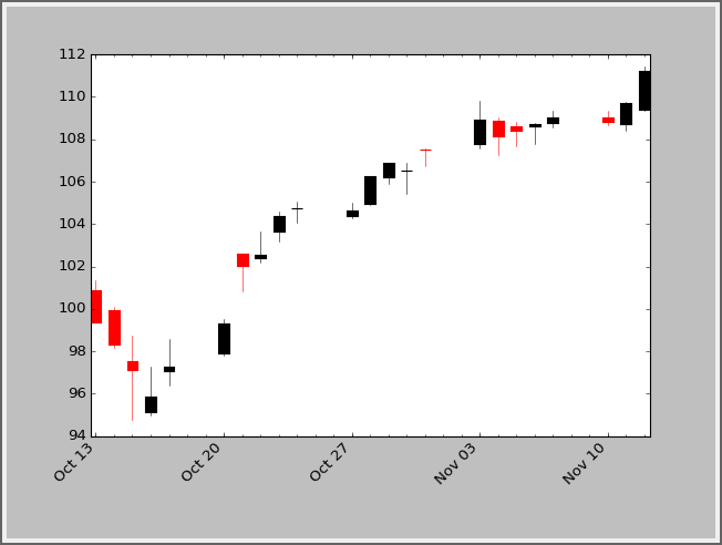
Candlestick chart
1 2 3 4 5 6 7 8 9 10 11 12 13 14 15 16 17 18 19 20 21 22 23 24 25 26 27 28 29 30 31 32 33 34 35 36 37 38 39 40 | """
Create a candlestick chart for a stock
"""
import matplotlib.pyplot as plt
from matplotlib.dates import DateFormatter, WeekdayLocator,\
DayLocator, MONDAY
from matplotlib.finance import quotes_historical_yahoo_ohlc, candlestick_ohlc
# Grab the stock data between these dates
date1 = (2014, 10, 13)
date2 = (2014, 11, 13)
# Go to the web and pull the stock info
quotes = quotes_historical_yahoo_ohlc('AAPL', date1, date2)
if len(quotes) == 0:
raise SystemExit
# Set up the graph
fig, ax = plt.subplots()
fig.subplots_adjust(bottom=0.2)
# Major ticks on Mondays
mondays = WeekdayLocator(MONDAY)
ax.xaxis.set_major_locator(mondays)
# Minor ticks on all days
alldays = DayLocator()
ax.xaxis.set_minor_locator(alldays)
# Format the days
weekFormatter = DateFormatter('%b %d') # e.g., Jan 12
ax.xaxis.set_major_formatter(weekFormatter)
ax.xaxis_date()
candlestick_ohlc(ax, quotes, width=0.6)
ax.autoscale_view()
plt.setp(plt.gca().get_xticklabels(), rotation=45, horizontalalignment='right')
plt.show()
|
There are many more things that can be done with matplotlib. Take a look at the thumbnail gallery: